Important Probability Distributions
Contents
1.4. Important Probability Distributions
An extensive collection of important probability distributions can be found on Wikipedia. In the following subsections, we will shortly review some of them.
1.4.1. Discrete Distributions
Note that each discrete probability distribution is completely described by the finite or countable sample space \(\Omega\) and the function \(p : \Omega \rightarrow [0, 1]\) which specifies the probability of each elementary event.
1.4.1.1. Bernoulli Distribution
The Bernoulli distribution \(\text{B}(1, p)\) is the distribution of a random variable \(X\) which takes only two possible values (usually encoded by \(0\) and \(1\)). The two values can be interpreted e.g. as false/true or failure/success. Thus,
and
For example, a coin flip can be modelled by a Bernoulli distribution. The outcome heads (\(X=1\)) has some probabiltity \(p \in [0, 1]\) and the outcome tails (\(X=0\)) has the complementary probability \(q = p - 1\). In the case of a fair coin, it holds \(p = 0.5\).
This distribution is of particular importance in machine learning with regard to binary classification.
1.4.1.2. Categorial Distribution
The categorial distribution is also called generalized Bernoulli distribution. Instead of only two different outcomes, it describes a random variable \(X\) with \(k\) different categories as outcomes (usually encoded by the numbers \(1, \dots, k\)). Each category \(i \in \{1, \dots, k\}\) possesses its individual probability
Note that the distribution is completely determined by \(k-1\) probabilities, since \(\sum_{i=1}^k p_i = 1\).
The distribution of a random variable for a fair dice is categorial with \(k=6\) and \(p_i = \frac{1}{6}\) for each \(k=1,\dots,6\). In this example, the categories (number of points) are ranked and the variable is called ordinal. Keep in mind that this kind of distribution also models cases with purely categorical observations (e.g., pictures of different pets) and in this case, \(i\) is simply a representation of some category, but it makes no sense to rank the categories.
This distribution is of particular importance in machine learning with regard to multiclass classification.
1.4.1.3. Binomial Distribution
The binomial distribution \(\text{B}(n, p)\) has two parameters \(n \in \mathbb{N}\) and \(p \in [0, 1]\). It describes the number of successes of \(n\) independent Bernoulli experiments with parameter \(p\). Thus, a random variable \(X\) with binomial distribution takes values \(\{0, \dots, n \}\) and
The binomial coefficient \({{n}\choose{k}}\) denotes the number of possibilities of exactly \(k\) successes in \(n\) independent Bernoulli trials.
For example, the probability of observing \(0\) heads in \(9\) flips of a fair coin is
1.4.1.4. Geometric Distribution
The geometric distribution \(\text{Geom}(p)\) describes the number of independent Bernoulli trials needed to get a success. Hence, it takes values in \(\{1, 2, \dots\}\) and
since \(X=k\) means no success in the first \(k-1\) Bernoulli trials (with probability \(1-p\) each) and finally a success in the \(k\)-th trial (with probability \(p\)). Note that \(P(X=k) \rightarrow 0\) as \(k \rightarrow \infty\) as long as \(p \ne 0\). For example, the probability to observe heads the first time after exactly \(10\) trials by tossing a fair coin is
Furthermore, in use of the third Kolmogorov axiom, it holds
In other words, the probability to observe only tails in the first \(9\) tosses is approximately \(0.02\%\) in correspondance with the calculation in use of the binomial distribution.
1.4.1.5. Poisson Distribution
The Poisson distribution \(\text{Pois}(\lambda)\) describes the distribution of a random variable \(X\) with values in \(\{0, 1, \dots \}\) and is given by
and some parameter \(\lambda > 0\). It models the number of events occuring in a fixed (time or space) interval if these events happen with a known constant mean rate and independently of each other. In fact, the expectation is \(\mathbb{E}(X) = \lambda\) and also \(\text{Cov}(X) = \lambda\). For example, the following scenarios can be modelled by a Poisson distribution:
radioactive decay: number of decays in a given time period of a radioactive sample
epidemiology: the number of cases of a disease in different cities
sports: the number of goals in a soccer match
If \(n\) is very large and \(p\) is very small the Poisson distribution can be used to approximate the binomial distribtion \(\text{B}(n, p)\) due to the Poisson limit theorem which is also called law of rare events.
1.4.2. Continuous Distributions
A continuous distribution is essentially specified by its probability density function.
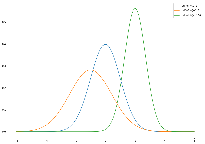
1.4.2.1. Normal Distribution
The multivariate normal distribution or Gaussian distribution \(\mathcal{N}(\mu, \Sigma)\) is the most important probability distribution with regard to the subsequent chapters. In particular, it is of special importance due to the central limit theorem.
The multivariate normal distribution is completely charaterized by its expectation \(\mu\) and covariance matrix \(\Sigma\). The general probability distribution function is given by
where \(\mu\) is some vector in \(\mathbb{R}^d\) and \(\Sigma\) is a symmetric and positive definite (i.e., \(x^T \Sigma x > 0\) for each \(0 \ne x \in \mathbb{R}^d\)) matrix. In particular, \(\Sigma^{-1}\) exists. Consequently, the univariate normal distribution (\(d=1\)) has the density
as well as \(\mu \in \mathbb{R}\) and \(\sigma^2 > 0\). Since
and
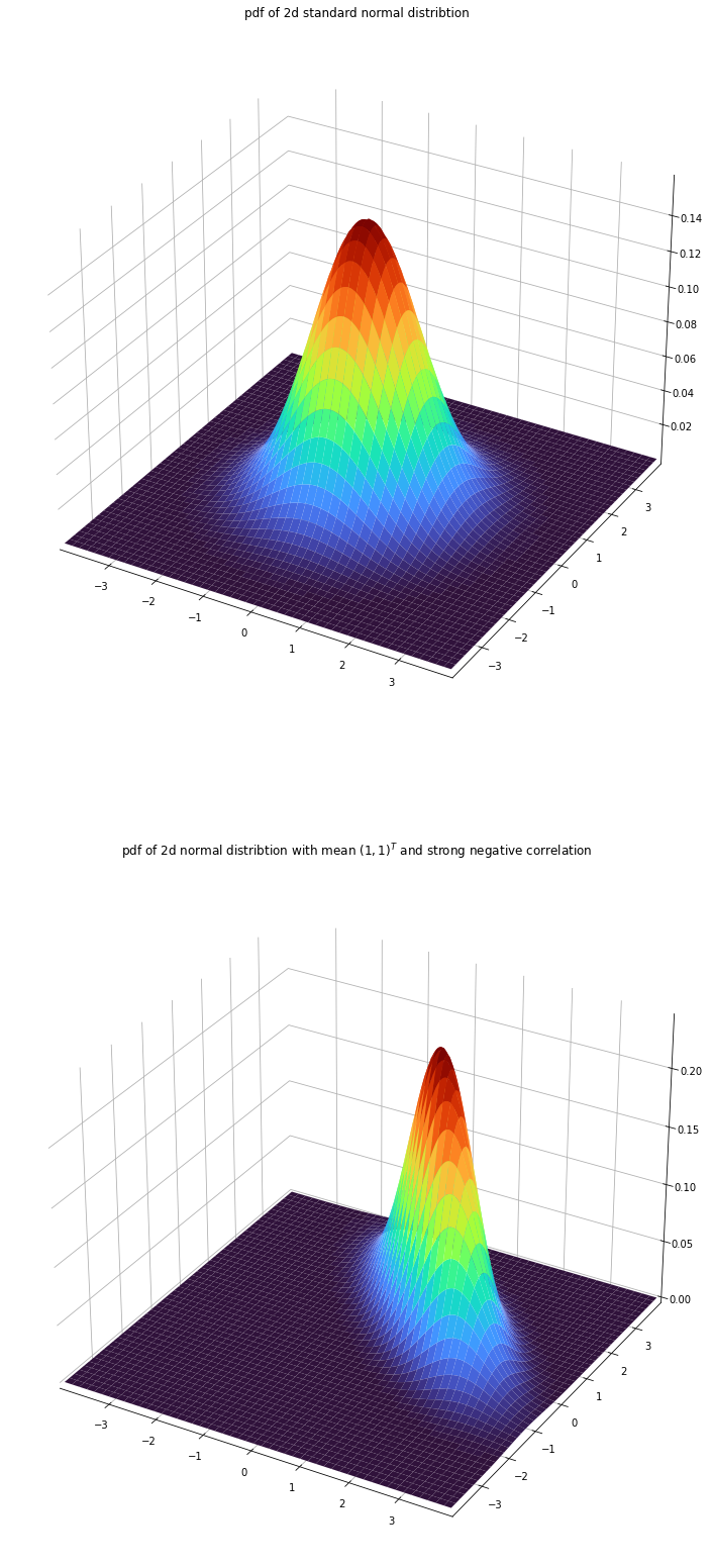
it holds \(\mathbb{E}(X) = \mu\) and \(\text{Cov}(X) = \sigma^2\) for a normally distributed random variable \(X\). This generalizes to the multivariate case, i.e.,
As mentioned before, in the case \(\mu = 0\) and \(\Sigma = I_d\) (identity matrix) we obtain the standard normal distribution.
import numpy as np
from scipy.stats import norm
import matplotlib.pyplot as plt

x = np.linspace(-6, 6, num=100)
plt.figure(figsize=(14, 10))
plt.plot(x, norm.pdf(x, loc=0, scale=1), label=r'pdf of $\mathcal{N}(0, 1)$')
plt.plot(x, norm.pdf(x, loc=-1, scale=np.sqrt(2)), label=r'pdf of $\mathcal{N}(-1, 2)$')
plt.plot(x, norm.pdf(x, loc=2, scale=np.sqrt(0.5)), label=r'pdf of $\mathcal{N}(2, 0.5)$')
leg = plt.legend()
import numpy as np
from scipy.stats import multivariate_normal
import matplotlib.pyplot as plt

def _adjust(ax):
    ax.xaxis.pane.fill = False
    ax.yaxis.pane.fill = False
    ax.zaxis.pane.fill = False
    ax.xaxis.pane.set_edgecolor('w')
    ax.yaxis.pane.set_edgecolor('w')
    ax.zaxis.pane.set_edgecolor('w')
    ax.set_xlim(-3.9, 3.9)
    ax.set_ylim(-3.9, 3.9)

x = np.linspace(-4, 4, 500)
y = np.linspace(-4, 4, 500)
X, Y = np.meshgrid(x,y)
tmp = np.stack((X, Y), axis=-1)
fig = plt.figure(figsize=(14, 28))
ax1 = fig.add_subplot(211, projection='3d')
_adjust(ax1)
ax1.plot_surface(X, Y, multivariate_normal.pdf(tmp, mean=[0, 0], cov = [[1, 0], [0, 1]]),
                cmap='turbo' ,linewidth=0)
t1 = ax1.set_title('pdf of 2d standard normal distribtion')
ax2 = fig.add_subplot(212, projection='3d')
_adjust(ax2)
p2 = ax2.plot_surface(X, Y, multivariate_normal.pdf(tmp, mean=[1, 1], cov = [[1, -0.75], [-0.75, 1]]),
                cmap='turbo' ,linewidth=0)
t2 = ax2.set_title(r'pdf of 2d normal distribtion with mean $(1, 1)^T$ and strong negative correlation')
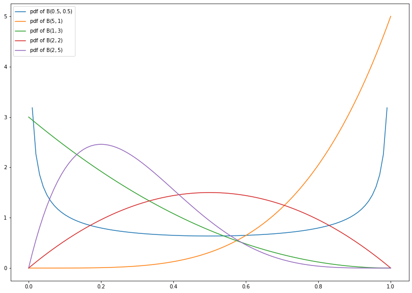
1.4.2.2. Beta Distribution
The beta distribution \(\text{Beta}(\alpha, \beta)\) is a continuous distribution with support on the interval \([0, 1]\), i.e., the probability of events outside \([0, 1]\) is zero. Its probability density function is given by
where \(\text{B}(\alpha, \beta) = \frac{\Gamma(\alpha) \Gamma(\beta)}{\Gamma(\alpha + \beta)}\) and \(\alpha, \beta > 0\). Here, \(\Gamma\) denotes the so-called Gamma function (an extension of the factorial).
import numpy as np
from scipy.stats import beta
import matplotlib.pyplot as plt

x = np.linspace(0, 1, num=100)
plt.figure(figsize=(14, 10))
plt.plot(x, beta.pdf(x, a=0.5, b=0.5), label=r'pdf of $\mathrm{B}(0.5, 0.5)$')
plt.plot(x, beta.pdf(x, a=5, b=1), label=r'pdf of $\mathrm{B}(5, 1)$')
plt.plot(x, beta.pdf(x, a=1, b=3), label=r'pdf of $\mathrm{B}(1, 3)$')
plt.plot(x, beta.pdf(x, a=2, b=2), label=r'pdf of $\mathrm{B}(2, 2)$')
plt.plot(x, beta.pdf(x, a=2, b=5), label=r'pdf of $\mathrm{B}(2, 5)$')
leg = plt.legend()
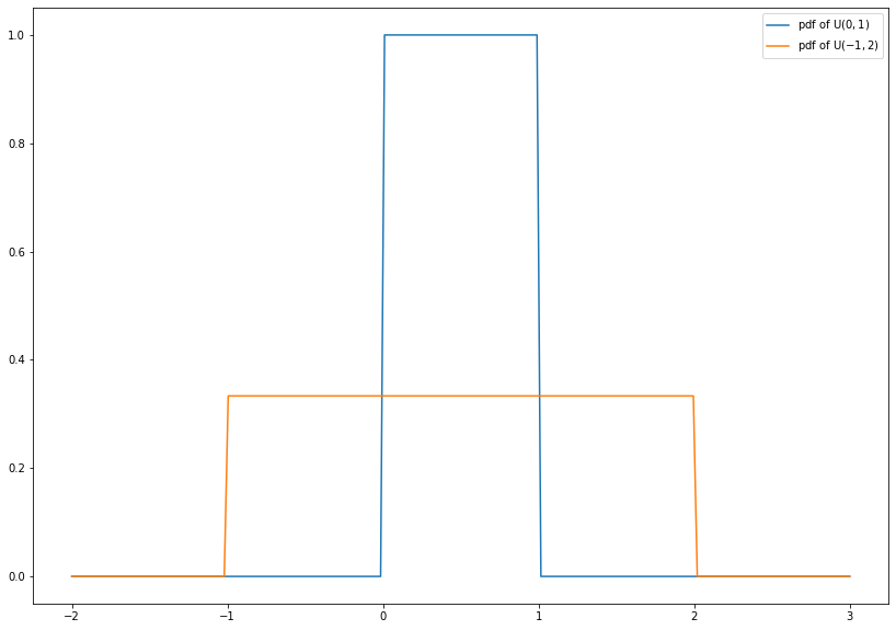
1.4.2.3. Uniform Distribution
The uniform distribtion \(\text{U}(a, b)\) is a continuous distribution with support \([a, b]\) for some numbers \(a < b\). It describes a random variable with arbitrary outcomes between \(a\) and \(b\). The probability density function reads
\(\text{U}(0, 1)\) is called standard uniform distribution. If a random variable \(X\) is \(\text{U}(0, 1)\)-distributed, then \(X^n\) is \(\text{Beta}(\frac{1}{n}, 1)\)-distributed. In particular, \(\text{U}(0, 1) = \text{Beta}(1, 1)\).
import numpy as np
from scipy.stats import uniform
import matplotlib.pyplot as plt

x = np.linspace(-2, 3, num=200)
plt.figure(figsize=(14, 10))
plt.plot(x, uniform.pdf(x, loc=0, scale=1), label=r'pdf of $\mathrm{U}(0, 1)$')
plt.plot(x, uniform.pdf(x, loc=-1, scale=3), label=r'pdf of $\mathrm{U}(-1, 2)$')
leg = plt.legend()
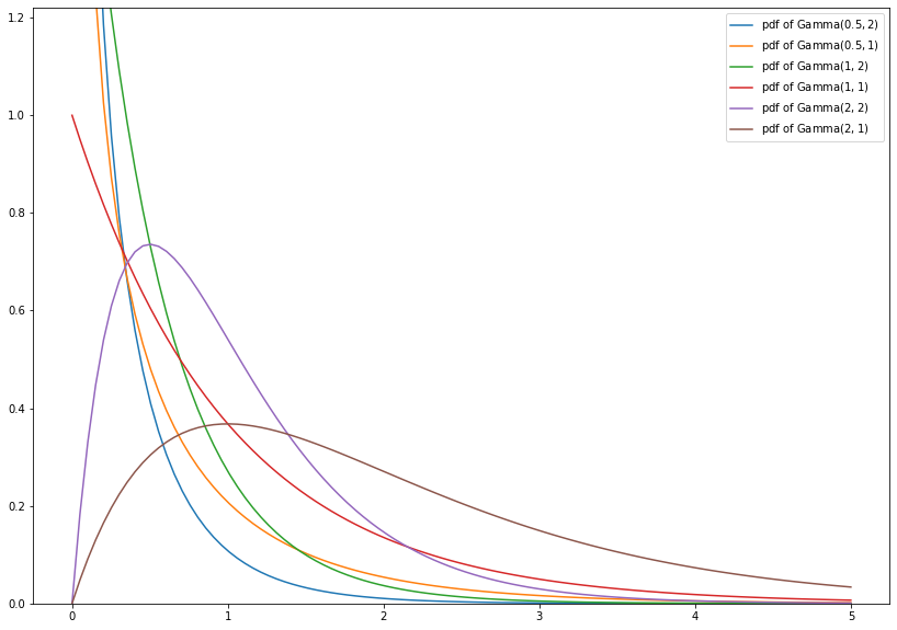
1.4.2.4. Gamma Distribution
The gamma distribution \(\text{Gamma}(\alpha, \beta)\) is a continuous probability distribution with support on \((0, \infty)\) which contains some important distributions as special cases. Its probability density function is given by
where \(\alpha, \beta > 0\).
import numpy as np
from scipy.stats import gamma
import matplotlib.pyplot as plt

x = np.linspace(0, 5, num=100)
plt.figure(figsize=(14, 10))
plt.plot(x, gamma.pdf(x, a=0.5, scale=0.5), label=r'pdf of $\mathrm{Gamma}(0.5, 2)$')
plt.plot(x, gamma.pdf(x, a=0.5, scale=1), label=r'pdf of $\mathrm{Gamma}(0.5, 1)$')
plt.plot(x, gamma.pdf(x, a=1, scale=0.5), label=r'pdf of $\mathrm{Gamma}(1, 2)$')
plt.plot(x, gamma.pdf(x, a=1, scale=1), label=r'pdf of $\mathrm{Gamma}(1, 1)$')
plt.plot(x, gamma.pdf(x, a=2, scale=0.5), label=r'pdf of $\mathrm{Gamma}(2, 2)$')
plt.plot(x, gamma.pdf(x, a=2, scale=1), label=r'pdf of $\mathrm{Gamma}(2, 1)$')
plt.ylim(0., 1.22)
leg = plt.legend()
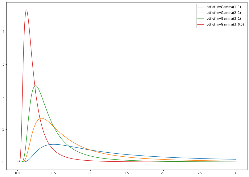
1.4.2.5. Inverse Gamma Distribution
The inverse gamma distribution \(\text{InvGamma}(\alpha, \beta)\) is a continuous probability distribution with support on \([0, \infty)\) and probability density function given by
where \(\alpha, \beta > 0\). Let \(X \sim \text{Gamma}(\alpha, \beta)\), then \(\frac{1}{X} \sim \text{InvGamma}(\alpha, \beta)\).
import numpy as np
from scipy.stats import invgamma
import matplotlib.pyplot as plt

x = np.linspace(0, 3, num=300)
plt.figure(figsize=(14, 10))
plt.plot(x, invgamma.pdf(x, a=1, scale=1), label=r'pdf of $\mathrm{InvGamma}(1, 1)$')
plt.plot(x, invgamma.pdf(x, a=2, scale=1), label=r'pdf of $\mathrm{InvGamma}(2, 1)$')
plt.plot(x, invgamma.pdf(x, a=3, scale=1), label=r'pdf of $\mathrm{InvGamma}(3, 1)$')
plt.plot(x, invgamma.pdf(x, a=3, scale=0.5), label=r'pdf of $\mathrm{InvGamma}(3, 0.5)$')
leg = plt.legend()
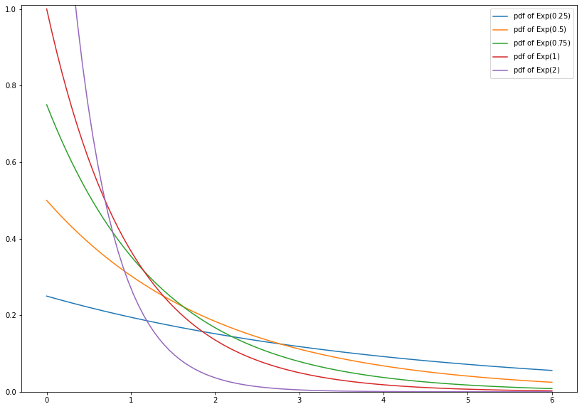
1.4.2.6. Exponential Distribution
The exponential distribution \(\text{Exp}(\lambda)\) is the continuous analogue of the geometric distribution. Its probability density function is given by
where \(\lambda > 0\). It holds \(\text{Exp}(\lambda) = \text{Gamma}(1, \lambda)\).
For example, the exponential distribution is used to model the time between two radioactive decays, i.e., the time between two random events which occur independently and at a constant average rate.
import numpy as np
from scipy.stats import expon
import matplotlib.pyplot as plt

x = np.linspace(0, 6, num=100)
plt.figure(figsize=(14, 10))
plt.plot(x, expon.pdf(x, scale=4), label=r'pdf of $\mathrm{Exp}(0.25)$')
plt.plot(x, expon.pdf(x, scale=2), label=r'pdf of $\mathrm{Exp}(0.5)$')
plt.plot(x, expon.pdf(x, scale=4/3), label=r'pdf of $\mathrm{Exp}(0.75)$')
plt.plot(x, expon.pdf(x, scale=1), label=r'pdf of $\mathrm{Exp}(1)$')
plt.plot(x, expon.pdf(x, scale=0.5), label=r'pdf of $\mathrm{Exp}(2)$')
plt.ylim(0., 1.01)
leg = plt.legend()
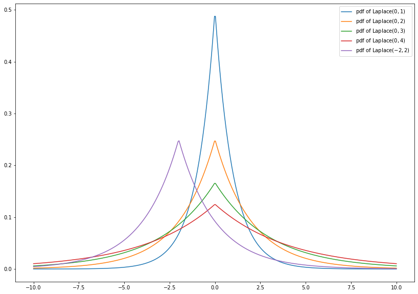
1.4.2.7. Laplace Distribution
The Laplace distribution \(\text{Laplace}(\mu, b)\) has the probability density function
where \(\mu \in \mathbb{R}\) and \(b > 0\).
Note that the density is a symmetric function around \(\mu\) and for \(x > \mu\) the density equals the pdf of a \(\text{Exp}(\frac{1}{b})\)-distribution (up to translation by \(\mu\)). For this reason, the Laplace distribution is also called double exponential distribution.
Moreover, the Lapalce distribution is similar to the normal distribution, but the squared difference to \(\mu\) in the exponential function is replace by the absolute difference.
import numpy as np
from scipy.stats import laplace
import matplotlib.pyplot as plt

x = np.linspace(-10, 10, num=400)
plt.figure(figsize=(14, 10))
plt.plot(x, laplace.pdf(x, loc=0, scale=1), label=r'pdf of $\mathrm{Laplace}(0, 1)$')
plt.plot(x, laplace.pdf(x, loc=0, scale=2), label=r'pdf of $\mathrm{Laplace}(0, 2)$')
plt.plot(x, laplace.pdf(x, loc=0, scale=3), label=r'pdf of $\mathrm{Laplace}(0, 3)$')
plt.plot(x, laplace.pdf(x, loc=0, scale=4), label=r'pdf of $\mathrm{Laplace}(0, 4)$')
plt.plot(x, laplace.pdf(x, loc=-2, scale=2), label=r'pdf of $\mathrm{Laplace}(-2, 2)$')
leg = plt.legend()
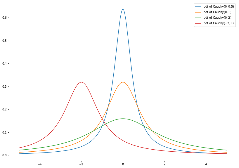
1.4.2.8. Cauchy Distribution
The Cauchy distribution \(\text{Cauchy}(x_0, \gamma)\) has probability density function
where \(x_0 \in \mathbb{R}\) and \(\gamma > 0\). \(\text{Cauchy}(0, 1)\) is also called standard Cauchy distribution and is the distribution of the ratio of two independent standard normally distributed random variables.
This distribution is well-known, since it does not have a well-defined mean and variance.
import numpy as np
from scipy.stats import cauchy
import matplotlib.pyplot as plt

x = np.linspace(-5, 5, num=400)
plt.figure(figsize=(14, 10))
plt.plot(x, cauchy.pdf(x, loc=0, scale=0.5), label=r'pdf of $\mathrm{Cauchy}(0, 0.5)$')
plt.plot(x, cauchy.pdf(x, loc=0, scale=1), label=r'pdf of $\mathrm{Cauchy}(0, 1)$')
plt.plot(x, cauchy.pdf(x, loc=0, scale=2), label=r'pdf of $\mathrm{Cauchy}(0, 2)$')
plt.plot(x, cauchy.pdf(x, loc=-2, scale=1), label=r'pdf of $\mathrm{Cauchy}(-2, 1)$')
leg = plt.legend()