Gaussian Process Classification
Contents
7.8. Gaussian Process Classification
Gaussian process are not only used for regression, but also for classification problems. Gaussian process classification uses a latent regression model to predict class probabilities. In a first step, we discuss binary classification and afterwards the setting is generalized to multiclass classification.
7.8.1. Binary Classification
In binary classification the data \(\mathcal{D}\) is of the form
i.e., the (discrete) label has either value \(-1\) or \(1\) representing the two possible classes. The sample matrix \(X\) and the lables \(y\) are constructed as before.
For a test point \(x^*\), the aim is to predict the class probabilities of the output \(y^*\), i.e., the probabilities \(p(y^*=1~|~X, y, x^*)\) and \(p(y^*=-1~|~X, y, x^*)\). In this way, we obtain one discrete probability distribution on \(\{-1, 1\}\) for each \(x^*\). Since
it is sufficient to focus on \(p(y^*=1~|~X, y, x^*)\). In other words, we are looking for a model which returns for a given input \(x^*\) the probability that the corresponding label is \(1\). For example, \(x^*\) could be an image which shows either a cat or a dog. The model has to quantify the probability for dog and the complementary probability yields the probability for cat. Certainly, we desire values close to 0 or 1, since values near 0.5 imply that the model has difficulties to classify the input.
It holds \(\sigma(z) \in [0,1]\), where
is the logistic response function.
%matplotlib inline
import numpy as np
from scipy.special import expit
import matplotlib.pyplot as plt
import seaborn as sns
sns.set_style('white')

fig = plt.figure(figsize=(14, 10))
x = np.linspace(-8, 8, num=100)
plt.plot(x, expit(x), label='logistic sigmoid')
leg = plt.legend(loc='lower right')
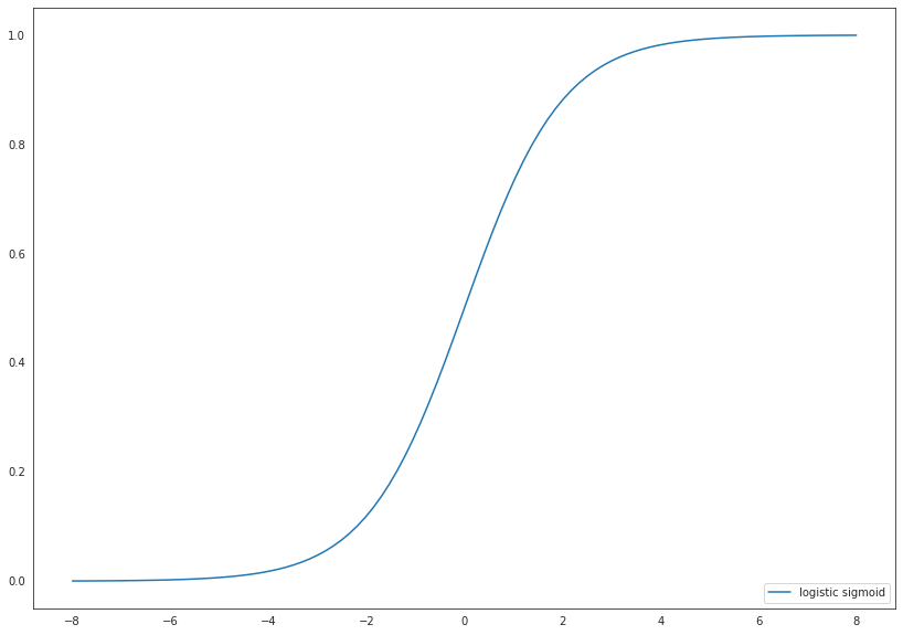
Hence, the value of \(\sigma(z)\) can be interpreted as a probability. It is also possible to use other response functions such as the Gaussian cdf, but we will restrict to \(\sigma\).
Our aim is to construct the distribution of a latent variable \(f^*\) given the data \(\mathcal{D}\) and a test point \(x^*\) (denote the pdf by \(p(f^*~|~X, y, x^*)\)) such that the class probability can be computed by the expectation of \(p(y^*=1~|~f^*) := \sigma(f^*)\):
Please note that \(p(y^*=-1~|~f^*) = 1 - p(y^*=1~|~f^*) = 1 - \sigma(f^*) = \sigma(-f^*)\) due to the properties of the logistic response function. Thus, the notation \(p(y^*~|~f^*) = \sigma(y^* f^*)\) is also used. Moreover, we like to mention that \(f^* < 0\) suggests that \(y^* = -1\) is more likely and vice versa \(f^* > 0\) implies that \(y^* = 1\) is more likely.
How can we construct \(p(f^*~|~X, y, x^*)\) in (7.5) by means of Gaussian process regression?
The answer to this question is rather complicated and technical. For the interested reader, we give the details in the subsequent part:
Explanation.
We follow the explanation in sections 3.3 and 3.4 of [1].
In Gaussian process regression we constructed a similar distribution \(p(f^*~|~X, f, x^*)\) representing the posterior over functions in terms of conditional distributions. Hence, the approach
is useful and natural, since it reduces the problem to determine the distribution of the latent labels \(f\) given the observations \(X\) and \(y\). Note that we denote the continuous labels by \(f\) instead of \(y\), since \(y\) is used for the discrete class labels.
At this point, it is already evident that Gaussian process classification is more challenging than regression. It is required to determine the pdf \(p(f~|~X, y)\) of an unobserved variable \(f\) and afterwards two integrals have to be calculated which involve the posterior distribution function of a Gaussian process regression model.
How can we compute \(p(f~|~X, y)\) in (7.6)?
Bayes’ theorem yields
since \(y\) depends by assumption only on the latent variable \(f\). In principle, we have all ingredients to create our classification model. Indeed, it holds
and
where \(p(f~|~X)\) is the marginal likelihood of the Gaussian process. Please note that we assume that the labels \(y\) are independent conditional on \(f\) in order to factorize in (7.8). However, the non-Gaussian likelihood \(p(y~|~f)\) makes it analytically intracable to compute the integral in (7.6).
Markov chain Monte Carlo (MCMC) methods are useful to compute the integrals. Another approach is the Laplace approximation of \(p(f~|~X, y)\) by a Gaussian distribution function \(q(f~|~X, y)\). The idea is to replace the unknown distribution by a suitable Gaussian distribution which is easier to handle. If we assume that \(p(f~|~X, y)\) would be indeed the pdf of a normal distribution, then mean and covariance would be given by
and
where \(\nabla\) and \(\nabla^2\) denote the first and second derivative, respectively. Thus, the Laplace approximation requires to find the maximum of a function depending on \(f\). For this purpose, we compute the roots of the gradient. The quality of the Laplace approximation depends of course on the shape of the real distribution function. For simplification of the calculation, we make to following changes:
instead of \(p(f~|~X, y)\) consider \(p(y~|~f) ~ p(f~|~X)\) in view of (7.7),
apply \(\ln\) to \(p(y~|~f) ~ p(f~|~X)\)
Thus, first \(p(f~|~X, y)\) is scaled by a constant and afterwards the strictly increasing function \(\ln\) is applied. A logarithmic transformation is useful, since it turns products into sums (which are easier to differentiate) and simplifies exponential terms. These modifications have no influence on the \(\text{argmax}\).
Set \(\Psi(f) := \ln \big(p(y~|~f) ~ p(f~|~X)\big)\). It holds
Thus, the gradient is given by
and the Hessian by
where \(W(f) := - \nabla^2 \ln \big(p(y~|~f)\big)\) is a diagonal matrix, since
\(\hat{f}\) fulfills \(\nabla \Psi(\hat{f}) = 0\) and hence, it holds
Unfortunately, \(\hat{f}\) also appears in the right-hand side of (7.11) and the equation can not be solved analytically. Therefore, another approximation is necessary. Roots of \(\nabla \Psi\) can be computed by Newton’s method in use of \(\nabla^2 \Psi\):
start with some initial value \(f_0\)
for \(i=0, 1, \dots\) compute iteratively
\[ f_{i+1} = f_i - \big(\nabla^2 \Psi(f_i)\big)^{-1} \nabla \Psi(f_i)\]until some stopping criterion is met
denote the result as \(\hat{f}\)
Thus, \(p(f~|~X, y)\) is replaced by the density \(q(f~|~X, y)\) of a \(\mathcal{N}(\hat{f}, \Sigma_{\hat{f}})\)-distributed random variable with
Consequently, the approximation of (7.6) yields
The integrand is the product of two probability distribution functions of normal distributions. Hence, \(q(f^*~|~X, y, x^*)\) is the density of a univariate normal distribution with mean
and variance
This result looks very familiar. Indeed, the mean and variance equal exactly the mean prediction and variance in Gaussian process regression with data given by \(X\) and \(\hat{f}\) as well as additional noise specified by \(W(\hat{f})^{-1}\).
For the sake of completeness, the derivation is presented in the following section:
Don’t do it!
For simplification of the notation, we write \(K := K(X, X)\) and \(W := W(\hat{f})\). It holds
and variance
since
The first summand in the integral yields the variance of the posterior Gaussian process distribution at \(x^*\). Recall that \(\mathbb{E}(f^*~|~X, f, x^*) = K(x^*, X)K^{-1}f\). Therefore, it follows
The last equation holds, since \(K^{-1} + K^{-1} \big(W + K^{-1}\big)^{-1} K^{-1} = \big(W^{-1} + K \big)^{-1}\) by
In order to compute the marginal likelihood \(p(y~|~X)\) the second order approximation
is used. To emphasize the dependence on the hyperparameters \(\theta\), we use the notation \(p(y~|~X, \theta)\) instead of \(p(y~|~X)\) and so forth. Note that \(\hat{f}\) and \(\Sigma_{\hat{f}}\) also depend on \(\theta\). It holds
Thefore, the log marginal likelihood reads
where \(K_{\theta}\) illustrates the dependence of \(K\) on \(\theta\) and \(B(X, \hat{f}) := K_{\theta}(X, X) {\Sigma_{\hat{f}}}^{-1}\). It holds
and thus, it follows
The last representation is particularly useful for implementation purposes, since \(I_n + W(\hat{f})^{\frac{1}{2}} K_{\theta}(X,X) W(\hat{f})^{\frac{1}{2}}\) is a positive definite matrix.
In application, the computational process can be summarized as follows:
Choose a Gaussian process with hyperparemeters \(\theta\) as prior for the latent labels \(f\)
For fixed \(\theta\) set \(\Psi(f) := \ln \big(p(y~|~f) ~ p(f~|~X, \theta)\big)\)
Compute the root \(\hat{f}\) (depends on \(\theta\)) of \(\nabla \Psi\) in use of Newton’s method
Calculate the log marginal likelihood by
\[\begin{split}\ln p(y~|~X, \theta) &\approx \ln \big(p(y~|~\hat{f})\big) - \frac{1}{2} \hat{f}^T K_{\theta}(X,X)^{-1} \hat{f} - \frac{1}{2} \ln \big(|K_{\theta}(X,X)|\big) + \frac{1}{2} \ln\big(|\Sigma_{\hat{f}}|\big)\\ &=\ln \big(p(y~|~\hat{f})\big) - \frac{1}{2} \hat{f}^T K_{\theta}(X,X)^{-1} \hat{f} - \frac{1}{2} \ln \big(|I_n + W(\hat{f})^{\frac{1}{2}} K_{\theta}(X,X) W(\hat{f})^{\frac{1}{2}}|\big),\end{split}\]where \(W(\hat{f}) = - \nabla^2 \ln \big(p(y~|~\hat{f})\big)\), \(\Sigma_{\hat{f}} = \big(W(\hat{f}) + K_{\theta}(X, X)^{-1}\big)^{-1}\) and
\[\ln \big(p(y~|~\hat{f})\big) = - \sum_{i=1}^n \ln \big(1 + \exp(-y_i\hat{f}_i)\big)\]Maximize \(\ln \big(p(y~|~X, \theta)\big)\) with respect to \(\theta\) (which means application of an optimization algorithm and looping steps 2.-4.)
Then, the class probability for a test point \(x^*\) in (7.5) is given by the one dimensional integral
where \(q(f^*~|~X, y, x^*)~df^*\) is the density of a normal distribution with mean
and variance
Thus, the assigned class probability is the expectation of \(\sigma\) with respect to the posterior distribution of the latent variable \(f^*\). If we are not interested in the precise value of the probability, but only in the favored class, it is sufficient to consider the sign of \(\mathbb{E}(f^*~|~X, y, x^*)\). For negative values the predicted class is \(-1\) and for positive values the predicted class is \(1\). This is equivalent to computing \(\sigma(\mathbb{E}(f^*~|~X, y, x^*))\) and to conclude that the predicted class is \(-1\) for a value less than \(0.5\) and the predicted class is \(1\) for a value larger than \(0.5\).
7.8.2. Multi-class Classification
In binary classification the data \(\mathcal{D}\) is of the form
i.e., the (discrete) label has either value \(-1\) or \(1\) representing the two possible classes. In the multi-class setting the data is of the form
where \(C_1, \dots, C_k\) represent the \(k\) different classes.
Similarly to the multi-output case in Gaussian process regression, several different approaches exist for multi-class classification. First of all, the Laplace approximtion discussed in Binary Classification can be generalized to a multi-class Laplace approximation (refer to Section 3.5 in [1]). Moreover, there exist general approaches to extend binary classifiers to multi-class tasks:
One-vs-Rest / One-vs-All:
\(k\) binary classifiers are trained by creating binary labels with the classes \(C_k\) (encoded as \(1\)) and all remaining classes (encoded as \(-1\))
For a test point each classifier predicts the probability for class \(C_k\) and the class with the highest probability is assigned
One-vs-One:
A binary problem is created by considering only two distinct classes \(C_k\) and \(C_l\), \(k \ne l\), (each possible pair of classes) and fitting a binary classifier (results in \(\frac{k~(k-1)}{2}\) classifiers)
Each model predicts a class probability and the class with most votes or alternatively, the class with the highest sum of probabilities is assigned
- 1(1,2)
C.E. Rasmussen and C.K.I. Williams. Gaussian Processes for Machine Learning. Adaptive Computation and Machine Learning. MIT Press, 2nd edition, 2006. URL: http://www.gaussianprocess.org/gpml/.