Coin Toss
3.1. Coin Toss
Imagine that we toss a coin multiple times and we would like to determine the probability to toss heads. Since this kind of random experiment has only two possible outcomes, the Bernoulli distribution \(\text{B}(1, \theta)\) is an appropriate model. The multiple coin tosses yield a sequence of indepdent random experiments. Each coin toss corresponds to a random variable \(X_i\) with value \(1\) for heads and value \(0\) for tails (\(X_i\) represents the \(i\)-th toss). Hence, we aim to determine \(\theta\). The sum \(\sum_i^n X_i\) describes the number of heads after \(n\) trials and has a binomial distribution \(\text{B}(n, \theta)\).
Let us assume that we doubt the fairness of the coin!
First, we use the frequentists approach which is strongly connected to the law of large numbers and the central limit theorem. Since we think the coin is not fair, we claim \(\theta \ne 0.5\).
Typically, we assume the opposite of our claim, i.e., the so-called null hypothesis
is assumed. The strategy is to find evidence that \(H_0\) is most likely wrong such that it is reasonable to reject the null hypothesis. In this way, we can accept our actual claim. This procedure is called hypothesis testing.
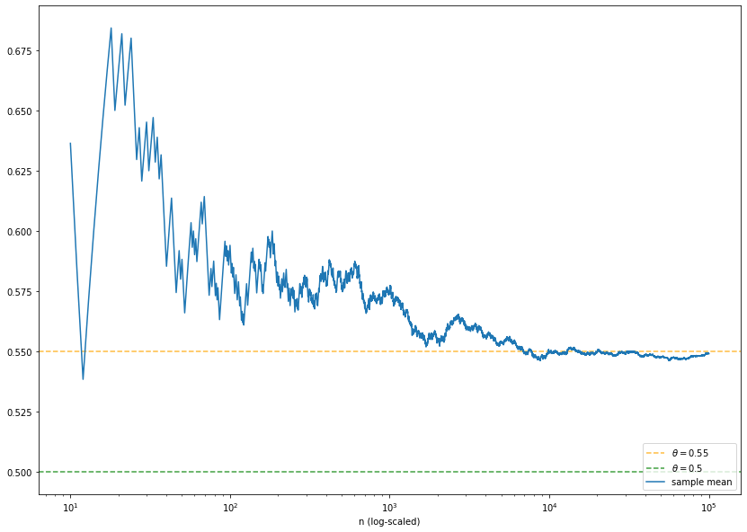
For each \(n \in \mathbb{N}\), the outcome of the average \(\overline{X}_n := \frac{1}{n} \sum_i^n X_i\) can be calulated (the sample mean \(\overline{x}_n\)). Due to the law of large numbers, we expect that this value approaches \(\theta\) for large values of \(n\). In any case, our estimate for \(\theta\) will differ at least slightly from the hypothesis \(\theta = 0.5\). From our frequentists point of view, we have to decide whether this difference is small enough to support the hypothesis. Maybe we should reject it? Under the assumption \(\theta=0.5\), we can approximate the distribution of \(\overline{X}_n\) by a normal distribution due to the central limit theorem and calculate a bound for the probability to observe the difference of the average to \(0.5\). The larger the difference the smaller the probability. This probability is called \(p\)-value. If the probability is smaller than a threshold of typically \(5\%\) , \(2\%\) or \(1\%\) , \(H_0\) is rejected. The correct interpretation is that our observation is not impossible if \(\theta=0.5\), but rather unlikely. Hence, we tend to conclude that \(\theta \ne 0.5\). The threshold is called significance level (denoted by \(\alpha\)). Note that the hypothesis test has a drawback: If e.g. \(\alpha = 5\%\), the nullhypothesis will be rejected by mistake in \(5\%\) of cases. This error is called type I error. At least, it is known how likely the type I error is and this error rate can be controlled by \(\alpha\). A type II error is the mistaken acceptance of the null hypothesis. In this case, the error rate is usually hard to determine.
So, let’s do the simulation:
import numpy as np
from scipy.stats import bernoulli, norm
import matplotlib.pyplot as plt

N = 100000 # total number of coin tosses
theta = 0.55 # probability to toss heads ("unknown")
theta0 = 0.5 # probability assumed in the null hypothesis
alpha_sig = 0.05 # significance level

# generate N independent B(1, theta)-distributed observations
samples = bernoulli.rvs(theta, size=N)

# caluclate the sample means after n=1,...,N trials
sample_sums = np.zeros((N,)) # for later use
sample_means = np.zeros((N,))
for n in range(N):
    sample_sums[n] = np.sum(samples[:n+1])
    sample_means[n] = sample_sums[n]/(n + 1)

# plot the result
fig = plt.figure(figsize=(14, 10))
plt.axhline(y=theta, color='orange', linestyle='--', alpha=.75, label=r'$\theta=${}'.format(theta))
plt.axhline(y=theta0, color='g', linestyle='--', alpha=.75, label=r'$\theta=${}'.format(theta0))
plt.xscale('log')
plt.xlabel('n (log-scaled)')
plt.plot(np.arange(10, N), sample_means[10:], label='sample mean')
leg = plt.legend(loc='lower right')

# perform the hypothesis test for selected values of n
n_values = np.arange(50, 2000, step=50)
n_tests = len(n_values)
upper_bounds = np.zeros(n_tests)
lower_bounds = np.zeros(n_tests)
for i, n in enumerate(n_values):
    sigma2 = theta0*(1-theta0)/n # variance of sample mean under H0
    upper_bounds[i] = norm.ppf(1-alpha_sig/2, loc=theta0, scale=np.sqrt(sigma2)) # upper bound of confidence interval
    lower_bounds[i] = 2*theta0 - upper_bounds[i] # lower bound of confidence interval

# plot the result
fig = plt.figure(figsize=(14, 10))
plt.errorbar(n_values, theta0*np.ones(n_tests), yerr=(upper_bounds - theta0),
             c='g', alpha=.75, fmt=':', capsize=3, capthick=1)
plt.fill_between(n_values, lower_bounds, upper_bounds, color='g', alpha=.25, label='confidence interval')
plt.xlabel('n')
plt.plot(n_values, sample_means[n_values], marker='.', c='b', label='sample mean')
leg = plt.legend()
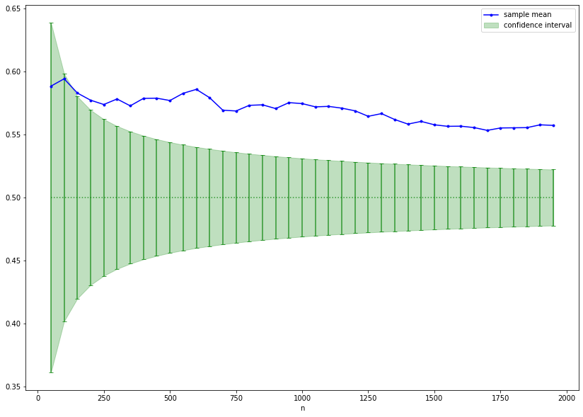
The confidence interval (green) illustrates the area around \(\theta=0.5\) such that the outcome of \(\overline{X}_n\) is inside the interval with probability \(1- \alpha\) supposed that \(0.5\) is the true value. If the sample mean (blue) is outside the confidence interval, the null hypothesis is rejected. Be careful! The interpretation that the true value of \(\theta\) is inside the confidence inerval with probability \(1- \alpha\) is wrong. In the frequentist setting the true value is either in the interval or it is not. This is not a question of probabilities. We can only be confident (up to some uncertainty given by \(\alpha\)) that the interval contains the outcome of \(\overline{X}_n\) under the assumption \(\theta=0.5\). This can be verified by simulating repeatedly a fixed number of tosses of a fair coin. In the long run, the sample mean should be inside the confidence interval in \(1- \alpha\) percent of the cases. This fact is nicely illustrated by an interactive visualization by Kristoffer Magnusson (please click on the image to follow the link):
Now, we analyze the problem the Bayesian way:
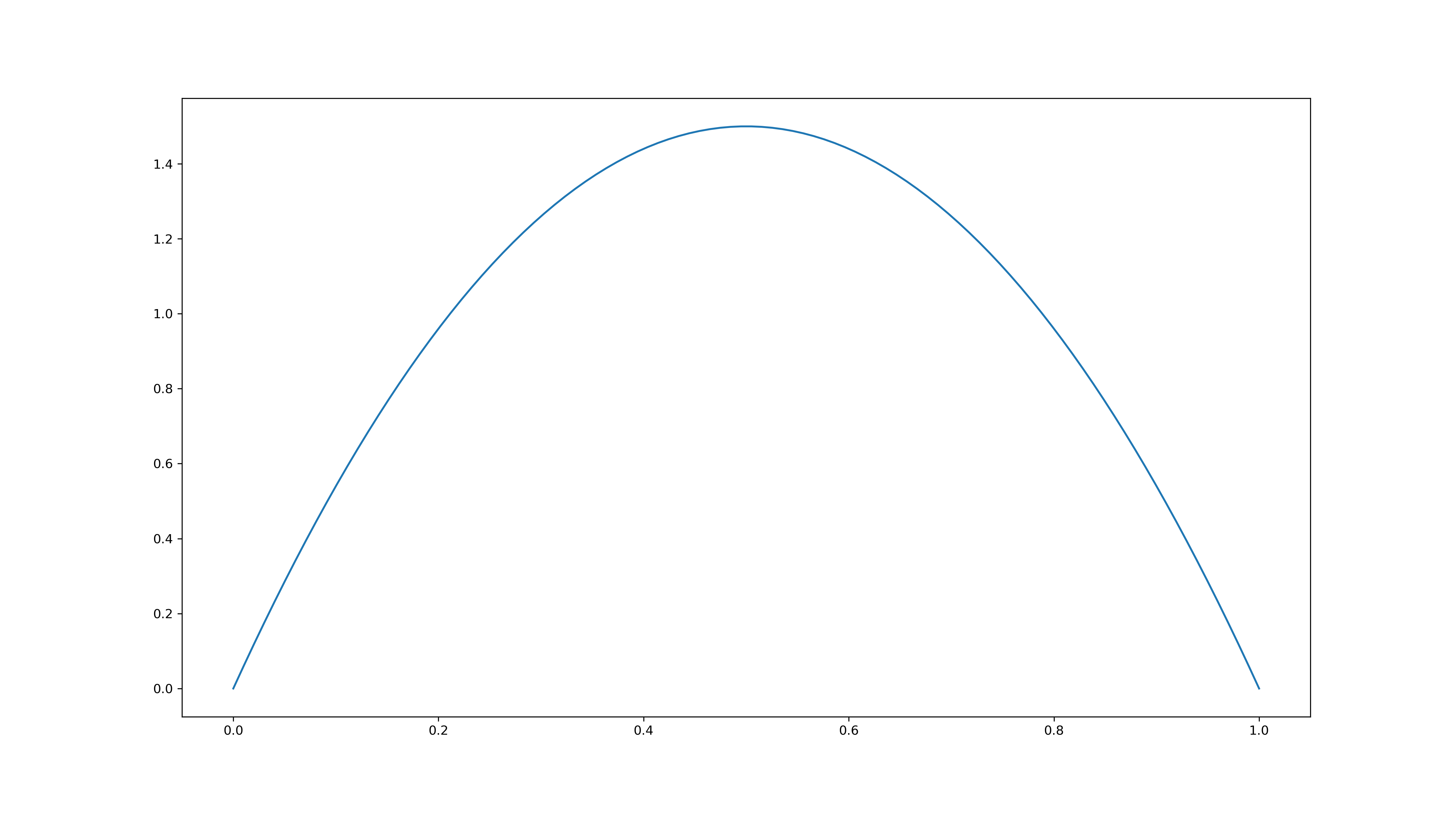
First, we include our prior beliefs on the value of \(\theta\). For this purpose, we assign a probability distribution to \(\theta\). Since \(\theta\) is itself a probability, the distribution should have support on \([0, 1]\). A good choice is the beta distribution \(\text{Beta}(\alpha, \beta)\). Suppose that we belief that our expectation is that \(\theta\) is near \(0.5\), but smaller or larger values are equally likely. Then, \(\alpha = \beta = 2\) is an appropiate choice and the prior distribution density looks like this:
Now, we do Bayesian inference. The goal is to update the distribution of \(\theta\) in use of observations. Instead of the sample mean \(\overline{x}_n\), we use the sample sum \(s_n\), since \(\sum_i^n X_i\) is \(\text{B}(n, \theta)\)-distributed. By Bayes’ theorem, it holds
The so-called evidence \(p(s_n)\) is independent of \(\theta\) and a normalization term which ensures that the righthand side is again a probability distribution.
\(p(\theta)\) is given by the prior distribution, i.e,
since we use \(\text{Beta}(2, 2)\) as prior distribution.
\(p(s_n~|~\theta)\) is called likelihood and is \(\text{B}(n, \theta)\)-distributed. Therefore, it holds
Consequently, it follows
where \(C\) is some constant (independent of \(\theta\)). This shows that the posterior distribution \(p(\theta~|~s_n)\) is again a beta distribution. More precisely, it is \(\text{Beta}(\alpha + s_n, \beta + n - s_n)\)-distributed. The observations yield an update of the distribution of \(\theta\), but it is always from the family of beta distributions. Note that \(\alpha\) and \(\beta\) (the choice of the prior) get less and less important as \(n\) increases.
The beta distribution is also called conjugate prior of the binomial distribution, since a beta distributed prior in combination with a binomial distributed likelihood yields a beta distributed posterior. This property enables sequential Bayesian inference, i.e., the posterior distribution can be used as prior distribution in the next inference step.
Let’s do the simulation:
import numpy as np
from scipy.stats import beta as beta_distr
import matplotlib.pyplot as plt
alpha = 2 # alpha of prior distribution
beta = 2 # beta of prior distribution
# use data (sample_sums) from first simulation
alphas = alpha + sample_sums # alpha values of posteriors
betas = beta + np.arange(1, N+1) - sample_sums # beta values of posteriors
# plot results for selected values of n
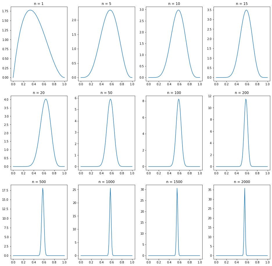
n_values = [1, 5, 10, 15, 20, 50, 100, 200, 500, 1000, 1500, 2000]
x = np.linspace(0, 1, num=100)
fig = plt.figure(figsize=(16, 16))
for i, n in enumerate(n_values):
ax = fig.add_subplot(3, 4, i+1)
ax.plot(x, beta_distr.pdf(x, alphas[n-1], betas[n-1]))
ax.title.set_text('n = {}'.format(n))
# compute confidence bounds of posterior distributions
n_values = np.arange(50, 2000, step=50)
n_tests = len(n_values)
posterior_means = np.array([alphas[n-1]/(alphas[n-1] + betas[n-1]) for n in n_values])
posterior_modes = np.array([(alphas[n-1] -1)/(alphas[n-1] + betas[n-1] - 2) for n in n_values])
lower_errors = []
upper_errors = []
for i, n in enumerate(n_values):
lower_errors.append(posterior_means[i] - beta_distr.ppf(alpha_sig/2, a=alphas[n-1], b=betas[n-1]))
upper_errors.append(beta_distr.ppf(1-alpha_sig/2, a=alphas[n-1], b=betas[n-1]) - posterior_means[i])
# plot results
fig = plt.figure(figsize=(14, 10))
plt.errorbar(n_values, posterior_means, np.array(list(zip(lower_errors, upper_errors))).T,
c='b', alpha=.75, fmt=':', capsize=3, capthick=1)
plt.fill_between(n_values, posterior_means - np.array(lower_errors), posterior_means + np.array(upper_errors),
color='b', alpha=.25, label='posterior credible interval')
plt.scatter(n_values, posterior_means, c='b', label='posterior mean')
# plt.scatter(n_values, posterior_modes, label='posterior mode')
plt.axhline(y=theta, color='orange', linestyle='--', alpha=.75, label=r'$\theta=${}'.format(theta))
plt.axhline(y=theta0, color='g', linestyle='--', alpha=.75, label=r'$\theta$={}'.format(theta0))
plt.xlabel('n')
leg = plt.legend()
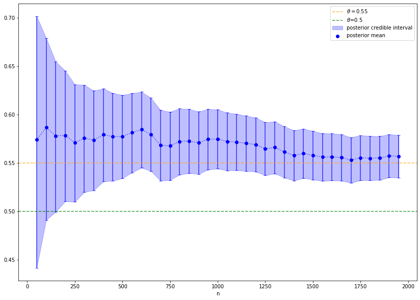
This approach yields the same conclusion: the coin is likely biased. Nevertheless, the way of thinking is different. In the first simulation, we supposed that it exist a true probability \(\theta\) for heads and came to the conclusion that \(\theta=0.5\) is an unlikely hypothesis and therefore, the hypothesis is rejected. In the second simulation, we do not prove a hypothesis true or false. Each value of \(\theta\) is still possible, but the posterior distributions shows that it is very likely to have a value larger than \(0.5\). In particular, it is possible to calculate probabilities with respect to the posterior distribution of \(\theta\). For example, in the above plot the value of \(\theta\) is in the so-called credible interval (blue) with probability \(1 - \alpha\). The Bayesian approach justifies to say that \(\theta\) is in the credible interval with a certain probability, since the probability reflects our beliefs on the value of \(\theta\).