7.10.1. Scalable Gaussian Processes¶

Recap Gaussian Process Regression

In GPR lemma we have fully discribed a Gaussian process for regression. We will shorten this notation of $K(X^*, X^*)$ to $K_{**}$ , $K(X^*, X)$ to $K_{*}^T$ and $K(X, X^*)$ to $K_{*}$, which leads to

\[\begin{split} \begin{aligned} p(y_* \lvert X_*X,y) &= \mathcal{N}(y_* \lvert \mu_*, \Sigma_*)\\ \mu_* &= K_{*}^T \big(K + \sigma_{\mathrm{noise}}^2 I_n\big)^{-1} y\\ \Sigma_* &= K_{**} - K_{*}^T \big(K + \sigma_{\mathrm{noise}}^2 I_n\big)^{-1} K_{*} \end{aligned} \end{split}\]

We can predict function values $f^*$ at new inputs $X^*$ with this. The most costly computation step of this is to compute the invserse of a covariance matrix (with noise)

\[ \big(K + \sigma_{\mathrm{noise}}^2 I_n\big)^{-1} \]

which is needed in the mean and the covariance of the gaussian process. This matrix has the size of $n \times n$, where $n$ is the number of training samples. The problem now is that, for large $n$ a matrix inversion is intractable.

The posterior can also be defined as

(7.12)¶\[\begin{align} p(f_* | X^*,X, y) &= \int p(f_*,f| X^*,X,y)df \quad \textrm{marginalize }f\\ p(f_* | X^*,X, y) &= \int p(f_*| X^*,X,f,y)p(f|X^*,X, y)df \quad \textrm{reserve chain rule}\\ p(f_* | X^*,X, y) &= \int p(f_* | X^*,X,f) p(f| X^*,X, y) df \quad \textrm{drop irrelevant y} \end{align}\]

Sparse Gaussian Process Regression

To avoid costly matrix inversion of $n \times n$-matrix, Authors in [2] propose to use the so called inducing variables. They assume the existence a set of $m$ inducing variables $f_m$ with corresponding inputs $X_m$ that will discribe our model well enough as if we used all datapoints $n$. Note that inducing variables $f_m$ evaluated at the pseudo-inputs $X_m$, which are independent from the training inputs. We will define the approximation posterior as $$ q(f_*) = \int p(f_* | f_m) \phi(f_m) df_m , $$

where $\phi(f_m)$ is the approximation of the intractable $p(f_m|y)$ and is defined by

\[ \phi(f_m) = \mathcal{N}(f_m | \mu_m, A_m). \]

Here is $\mu_m$ the mean and $A_m$ the covariance matrix. The goal is to find optimal values for the mean $\mu_m$ and covarince $A_m$ as well as the optimal location of the inducing inputs $X_m$. The mean and covariance matrix of the Guassian Process is defined by

(7.13)¶\[\begin{align} q(f_*) =& \mathcal{N}(f_* | \mu_*^q, \Sigma_*^q) \\ \mu_*^q =& K_{*m} K_{mm}^{-1} \mu_m \\ \Sigma_*^q =& K_{**} - K_{*m} K_{mm}^{-1} K_{m*} + K_{*m} K_{mm}^{-1} \mathbf{A}_m K_{mm}^{-1} K_{m*} \end{align}\]

where $K_{mm}=K(X_m,X_m)$, $K_{*m}=K(X_*,X_m)$ and $K_{m*}=K(X_m,X_*)=K_{*m}^T$. Now we can see, that we have to do the inversion of a $m \times m$ matrix if we found the optimal values for $\mu_m, A_m$ and $X_m$. For optimization of this we will use a variational approach by minimizing the Kullback-Leibler (KL) divergence between the approximate $q(f)$ and the exact posterior $p(f|y)$ over latent variables $f$.

The minimization of KL divergence is equivalent to maximization of a lower bound $\mathcal{L}(\mu_m, A_m,X_m)$ on the true log marginal likelihood $\log p(y).$ This lower bound can be optimized by analytically solving for $μ_m$ and $A_m$. The resulting lower bound after optimization is a function of $X_m$:

\[ \mathcal{L}(X_m)= \log \mathcal{N}(y|0,\sigma^2_y I+ Q_{nn})-\frac{1}{2 \sigma^2_y}\textrm{Tr}(K_{nn}-Q_{nn}) \]

with $Q_{nn}=K_{nm}K_{mm}^{-1}K_{mn}$. The first term on the RHS is the approximate log likelihood term and the second one is a regularization term which result of using variational approach.The second term can be interpreted as minimizing the error predicting $f$ from inducing variables $f_m$. The better the variables $f_m$ represent the function to be modeled the smaller this error will be. So the optimization will try to find the best postions for the inducing inputs $X_m$. With optimal inducing inputs $X_m$ we ca analytically find values for $\mu_m$ and $A_m$.

\[ \mu_m = \frac{1}{\sigma_y^2} K_{mm} \Sigma K_{mn} y \]

\[ A_m = K_{mm} \Sigma K_{mm} \]

where $\Sigma = (K_{mm}+\sigma^2_yK_{mm}K_{nm}^{-1})$ is.

For a more detailed description of sparse and variational GP, please refer to [1].

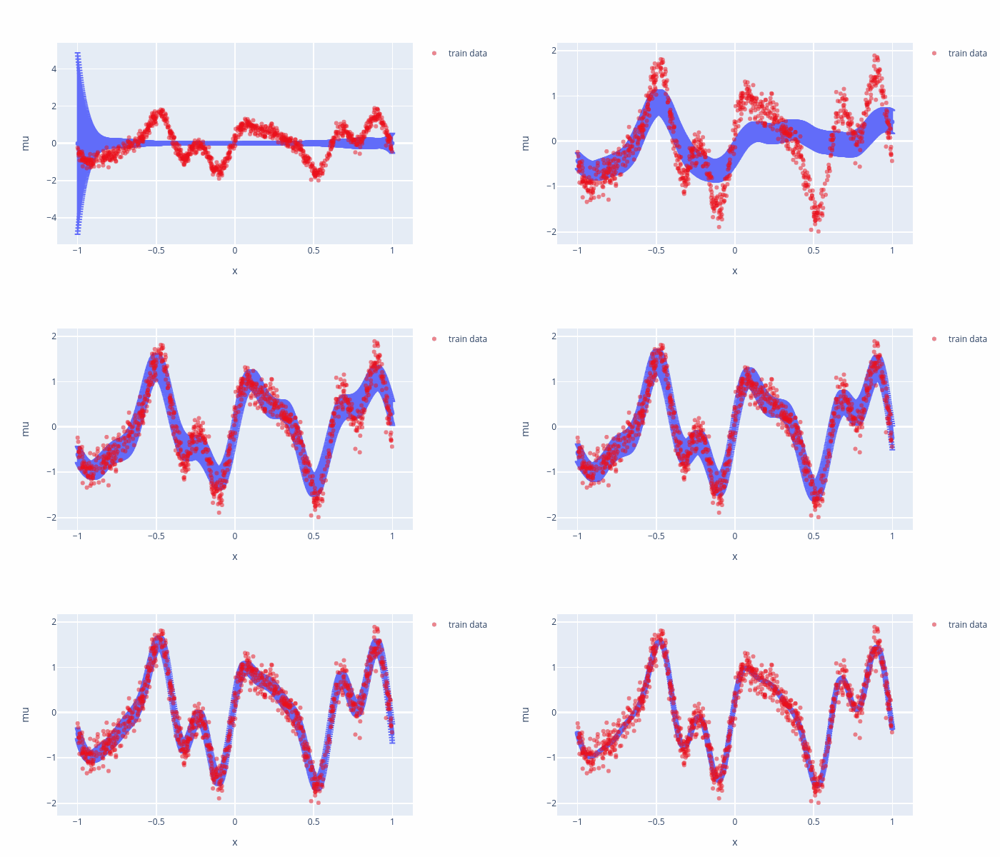
Visualization of SVGP training

Fig. 7.1 Evolution of the inducing points.¶

Fig. 7.2 Evolution of the model points displayed as $\mu_*\pm 2\sigma_*^2$¶

As the training goes on, some inducing points are moved outside of the training boundaries and their values are set to mean ($0$) which relating to a small variance where we do not have any datapoints. To avoid such a behavior, we can set “whiten = True” the SVGP, which a variable transformation and should not effect the model.

import numpy as np
from sklearn.datasets import fetch_california_housing
from sklearn.model_selection import train_test_split
from sklearn.preprocessing import StandardScaler, MinMaxScaler
from sklearn.decomposition import PCA
from sklearn.gaussian_process import GaussianProcessRegressor
from sklearn.gaussian_process.kernels import RBF, Matern, ConstantKernel, WhiteKernel
from sklearn.metrics import r2_score, mean_squared_error, mean_absolute_error
import gpflow
import tensorflow as tf
import matplotlib.pyplot as plt
from gpflow.ci_utils import ci_niter
import time


# load data
housing_dataset = fetch_california_housing()

# use first feature (median income) as additional label
X = housing_dataset["data"]#[:, 1:]
#y = np.stack((housing_dataset["target"], housing_dataset["data"][:, 0]), axis=1)
y = housing_dataset["target"].reshape(-1, 1) #als Übung
# split data (50% train and 50% test)
# training: 10320 samples, test: 10320 samples
X_train, X_test, y_train, y_test = train_test_split(X, y, test_size=0.5, random_state=42)

# scale data
scalerX, scalery = StandardScaler(), StandardScaler()
X_train_ = scalerX.fit_transform(X_train)
y_train_ = scalery.fit_transform(y_train)

N = len(X_train_)

rng = np.random.RandomState(123)
tf.random.set_seed(42)


X = X_train_
Y = y_train_ 
data = (X, Y)


# Choose equidistance locations for initial values for inducing locations.
M = 5  # Number of inducing locations
idx = [int(i) for i in list(np.linspace(0, N, M, endpoint=False))]
Z = X[idx, :].copy()  # Initialize inducing locations to the first M inputs in the dataset


# Create SVGP model.
start_time = time.time()
kernel = gpflow.kernels.SquaredExponential()

# whiten=True toggles the fₛ=Lu parameterization.
# whiten=False uses the original parameterization. see e.g.: https://towardsdatascience.com/sparse-and-variational-gaussian-process-what-to-do-when-data-is-large-2d3959f430e7
m = gpflow.models.SVGP(kernel, gpflow.likelihoods.Gaussian(), Z, num_data=N, whiten=True)
# Enable the model to train the inducing locations.
gpflow.set_trainable(m.inducing_variable, True)

# Set batch size.
minibatch_size = 100
train_dataset = tf.data.Dataset.from_tensor_slices((X, Y)).repeat().shuffle(N)

def run_adam(model, iterations):
    """
    Utility function running the Adam optimizer
    :param model: GPflow model
    :param interations: number of iterations
    """
    # Create an Adam Optimizer action
    logf = []
    train_iter = iter(train_dataset.batch(minibatch_size))
    training_loss = model.training_loss_closure(train_iter, compile=True)
    optimizer = tf.optimizers.Adam()

    @tf.function
    def optimization_step():
        optimizer.minimize(training_loss, model.trainable_variables)

    for step in range(iterations):
        optimization_step()
        if step % 1000 == 0:
            elbo = -training_loss().numpy()
            print(step, elbo)
            logf.append(elbo)
    return logf

# Specify the number of optimization steps.
maxiter = ci_niter(30000)

# Perform optimization.
logf = run_adam(m, maxiter)

-20222.25999866008
-14482.374430027356
-13003.58781728674
-10188.432377988136
-11492.638190511052
-12639.439790135742
-10170.374511297925
-9522.218133477993
-10660.730242307336
-10301.516341396069
-10159.830518487901
-7729.894608357307
-10375.753024366632
-10936.726274038821
-10213.366064974267
-9772.123785135893
-11289.154383840001
-8683.425254500584
-9472.522113928679
-10802.898018417705
-10695.549488236797
-8464.78685919514
-10073.512543821193
-7624.815088496258
-10690.345525680475
-12232.215858685458
-8769.56863686641
-8991.181014518046
-11150.114254287839
-12494.928158969995

# test model
y_pred ,y_pred_v = m.predict_y(scalerX.transform(X_test))
#y_pred = pca.inverse_transform(y_pred)
y_pred = scalery.inverse_transform(y_pred)
#y_pred = np.rint(y_pred) # labels should be integer valued
r2 = r2_score(y_test, y_pred)
mse = mean_squared_error(y_test, y_pred)
mae = mean_absolute_error(y_test, y_pred)
print("---SVGP execution in %s seconds ---" % (time.time() - start_time))
print("\nr2 = {:.4f}, mse = {:.2f}, mae = {:.2f}".format(r2, mse, mae))

--- 36.33657693862915 seconds ---

r2 = 0.6395, mse = 0.48, mae = 0.51

1: Felix Leibfried, Vincent Dutordoir, ST John, and Nicolas Durrande. A tutorial on sparse gaussian processes and variational inference. 2021. arXiv:2012.13962.
2: Michalis Titsias. Variational learning of inducing variables in sparse gaussian processes. In David van Dyk and Max Welling, editors, Proceedings of the Twelth International Conference on Artificial Intelligence and Statistics, volume 5 of Proceedings of Machine Learning Research, 567–574. Hilton Clearwater Beach Resort, Clearwater Beach, Florida USA, 16–18 Apr 2009. PMLR. URL: https://proceedings.mlr.press/v5/titsias09a.html.

Introduction to Probabilistic Machine Learning

Scalable Gaussian Processes

7.10.1. Scalable Gaussian Processes¶