3.3. MAP and MLE¶

In Bayesian Inference, we have seen that the main task is to compute the posterior distribution by

\[p(\theta~|~\mathcal{D}) = \frac{p(\mathcal{D}~|~\theta)~p(\theta)}{p(\mathcal{D})}.\]

Note that \(p(\theta~|~\mathcal{D})\) is a probability density function depending on \(\theta\). If the expression on the righthand side is not computable, an alternative is required. A useful approach is to use the mode \(\hat{\theta}\) of the posterior distribution:

\[\hat{\theta} := \underset{\theta}{\text{argmax}} ~ p(\theta~|~\mathcal{D}) = \underset{\theta}{\text{argmax}} ~ \frac{p(\mathcal{D}~|~\theta)~p(\theta)}{p(\mathcal{D})} = \underset{\theta}{\text{argmax}} ~ p(\mathcal{D}~|~\theta)~p(\theta)\]

The denominator can be neglected, since \(p(\mathcal{D})\) does not depend on \(\theta\). Roughly speaking, the most likely value of \(\theta\) with respect to the posterior distribution is used. This method is called maximum a-posteriori method (MAP). A special case of the MAP method results by using a uniform prior distribution for \(\theta\). In this case, each value for \(\theta\) is a priori assumed to be equally likely which means that no prior knowledge is imposed. This method is called maximum likelihood estimation (MLE):

\[\hat{\theta} = \underset{\theta}{\text{argmax}} ~ p(\mathcal{D}~|~\theta)\]

As the name suggests, MLE coincides with maximization of the likelihood \(p(\mathcal{D}~|~\theta)\).

The MAP estimate \(\hat{\theta}\) also enables to make predicitions for new data points in use of \(p(x ~|~\hat{\theta})\).

Please note that these methods are not Bayesian in the proper sense, since the distribution of \(\theta\) is replaced by a fixed value.

In the coin toss example with \(\text{Beta}(\alpha, \beta)\) prior distribution, we have seen that \(p(\theta~|~\mathcal{D})\) is \(\text{B}(\alpha + s_n, \beta + n - s_n)\)-distributed. Therefore, the MAP estimate is given by the mode of this beta distribution which equals

\[\hat{\theta} = \frac{\alpha + s_n - 1}{\alpha + \beta + n -2}.\]

Moreover, for \(\alpha = \beta = 1\) the prior distribution equals a uniform distribution and hence, the MAP estimate yields the MLE value for \(\hat{\theta}\). As seen before, in this example \(\hat{\theta}\) equals also the probability for heads, since it is the parameter of a Bernoulli distribution. In Bayesian Inference, we have seen that the full Bayesian inference and use of the posterior predictive distribution yields that the probability for heads equals the expectation of the beta distribution which differs from its mode. Indeed, it holds

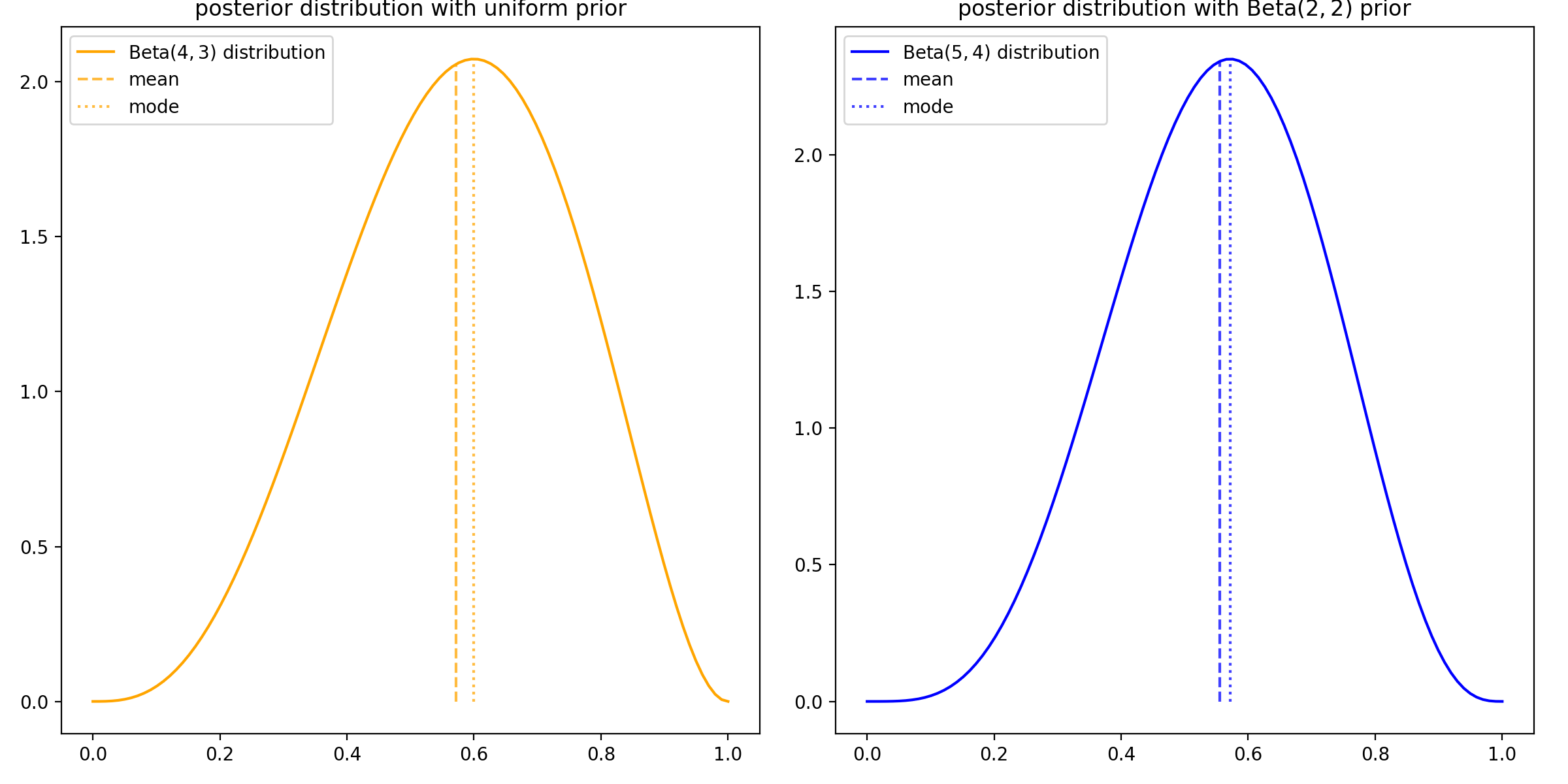
\[\begin{split} P(H~|~\mathcal{D}) = \begin{cases} \frac{\alpha + s_n}{\alpha + \beta + n}, & \text{in use of full Bayesian inference} \\ \frac{\alpha + s_n - 1}{\alpha + \beta + n -2}, & \text{in use of the MAP estimate} \end{cases} \end{split}\]

Assuming again the five coin tosses with 3 heads and 2 tails, the following values for \(P(H~|~\mathcal{D})\) result from the different approaches and priors:

	uniform prior	\(B(2, 2)\) prior
Bayesian inference (mean)	\(\frac{4}{7} \approx 0.57\)	\(\frac{5}{9} \approx 0.56\)
MAP (mode)	\(\frac{3}{5} = 0.6\)	\(\frac{4}{7} \approx 0.57\)

The differences are illustrated in the following plot:

Introduction to Probabilistic Machine Learning

MAP and MLE

3.3. MAP and MLE¶